How do I filter a PivotTable based on cell value?

Filter Items based on Value

1. Go to Row Label filter –> Value Filters –> Greater Than.
2. In the Value Filter dialog box: Select the values you want to use for filtering. In this case, it is the Sum of Sales (if you have more items in the values area, the drop down would show all of it). Select the condition. ...
3. Click OK.

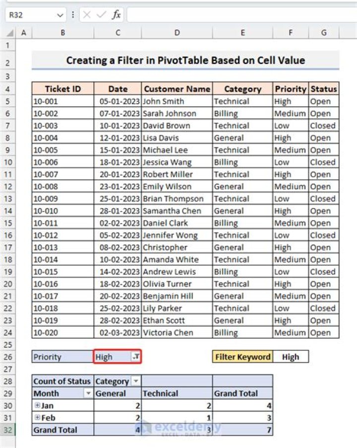
Can I use a cell reference to filter a pivot table?

YES it's very much possible that you can use a Cell Reference to Filter records while using the Pivot Table.

How do I filter a pivot table based on a list?

The quickest way to see a list of the Multiple Items in the filter is to add a slicer to the pivot table.

1. Select any cell in the pivot table.
2. Select the Analyze/Options tab in the ribbon.
3. Click the Insert Slicer button.
4. Check the box for the field that is in the Filters area with the filter applied to it.
5. Press OK.

How do I filter a pivot table based on multiple cell values in Excel?

Change the Pivot Table Filter Options

1. Right-click a cell in the pivot table, and click PivotTable Options.
2. Click the Totals & Filters tab.
3. Under Filters, add a check mark to 'Allow multiple filters per field. '
4. Click OK.

How do I filter multiple values in a pivot table?

Right-click a cell in the pivot table, and click PivotTable Options. Click the Totals & Filters tab Under Filters, add a check mark to 'Allow multiple filters per field. ' Click OK.

How can one filter a PivotTable using a report filter?

How can one filter a PivotTable using a report filter? a. Click the Report Filter's drop-down arrow, then click on an item to select an item in the list and click OK.

How do you link a filter to a cell?

To apply a filter for a cell's value:

1. Right-click a cell that contains the value you want to filter for.
2. Choose Filter > Filter by Selected Cell's Value.
3. The filter will be applied to the column.

How do I add a filter to a cell in Excel?

How to add filter in Excel

1. On the Data tab, in the Sort & Filter group, click the Filter button.
2. On the Home tab, in the Editing group, click Sort & Filter > Filter.
3. Use the Excel Filter shortcut to turn the filters on/off: Ctrl+Shift+L.

How do I filter data in Excel?

To filter with search:

1. Select the Data tab, then click the Filter command. A drop-down arrow will appear in the header cell for each column. ...
2. Click the drop-down arrow for the column you want to filter. ...
3. The Filter menu will appear. ...
4. The worksheet will be filtered according to your search term.

What is calculation in PivotTable?

In PivotTables, you can use summary functions in value fields to combine values from the underlying source data. If summary functions and custom calculations do not provide the results that you want, you can create your own formulas in calculated fields and calculated items.

How do I drop report filter fields here?

To show the Report Filters across the row:

1. Right-click a cell in the pivot table, and click Pivot Table Options.
2. On the Layout & Format tab, click the drop down arrow beside 'Display Fields in Report Filter Area'
3. Click 'Over, Then Down'

How do you change a summary to a average?

1. Select a field in the Values area for which you want to change the summary function of the PivotTable report.
2. On the Options tab, in the Active Field group, click Active Field, and then click Field Settings. ...
3. Click the Summarize Values By tab.

How do you remove the commissions filter from this PivotTable?

icon to the left of the arrow.

1. In the design window, make sure the PivotTable list is activated. For instructions, see Help for your design program.
2. Do one of the following: Remove all filters. Click the AutoFilter button. on the toolbar so that it is not selected. Note If you click AutoFilter.

What is the recommended way to create a new PivotTable style that is close to an existing style?

Create a New PivotTable Style

• Select a cell in the pivot table, and on the Ribbon, click the Design tab.
• In the PivotTable Styles gallery, click New PivotTable Style (at the bottom of the PivotTable Styles gallery)

How do I use advanced filter in PivotTable?

Whatever you want to filter your pivot tables by (in Jason's situation, it's type of beer), you'll need to apply that as a filter. Click within your pivot table, head to the “Pivot Table Analyze” tab within the ribbon, click “Field List,” and then drag “Type” to the filters list.

How do I create a filtered data PivotTable?

Create the Pivot Table

1. Insert a new sheet, and name it PivotVis.
2. Select any cell on the new sheet.
3. On the Excel Ribbon, click the Insert tab.
4. Click the Pivot Table command.
5. In the Create PivotTable dialog box, click in the Table/Range box, and press the F3 key on your keyboard.

How do I remove grand total from PivotTable in Excel?

Show or hide grand totals

Click anywhere in the PivotTable to show the PivotTable Analyze and Design tabs. Click Design > Grand Totals. Pick the option you want: Off for Rows & Columns.

Which KPI field should you add to a PivotTable If you want to display the KPI icon?

The KPI indicator appears as another type of field you can insert into the quadrants in the associated PivotTable. You can insert the “Value,” “Goal,” or “Status” of the KPI into the “Values” quadrant in the “PivotTable Fields” task pane.

How do you put a grand total in a calculated field in a PivotTable?

Click the PivotTable. On the Analyze tab, in the PivotTable group, click Options. In the PivotTable Options dialog box, on the Totals & Filters tab, do one of the following: To display grand totals, select either Show grand totals for columns or Show grand totals for rows, or both.

How do I filter multiple columns based on single criteria in Excel?

To filter with search:

1. Select the Data tab, then click the Filter command. A drop-down arrow will appear in the header cell for each column. ...
2. Click the drop-down arrow for the column you want to filter. ...
3. The Filter menu will appear. ...
4. When you're done, click OK. ...
5. The worksheet will be filtered according to your search term.

What is Advanced Filter in Excel?

More Information. The Advanced Filter gives you the flexibility to extract your records to another location on the same worksheet or another worksheet in your workbook. It also allows the use of an "OR" statement in your Filters. ( Example: Which sales were less than $400 "OR" greater than $600).

How do I filter multiple values in one column in Excel?

Select Filter the list, in-place option from the Action section; (2.) Then, select the data range that you want to filter in the List range, and specify the list of multiple values you want to filter based on in the Criteria range; (Note: The header name of the filter column and criteria list must be the same.) 3.